Customer First Order Segmentation using Looker and Google BigQuery — Rittman Analytics
Along with Recency, Frequency and Monetary Value (RFM) segmentation, one of the most valuable and actionable ways that you can segment your customers is by the first, last and most frequent products and services they order.
The product a customer first orders from you is usually a good predictor of customer persona and, for example, their likelihood to go on and make more purchases.
The amount a customer spends on their first order is often a good predictor of the amount they’ll spend with you over their lifetime.
Channels that bring in customers who over time become your most valuable customers are the channels you should focus your future marketing budget on.
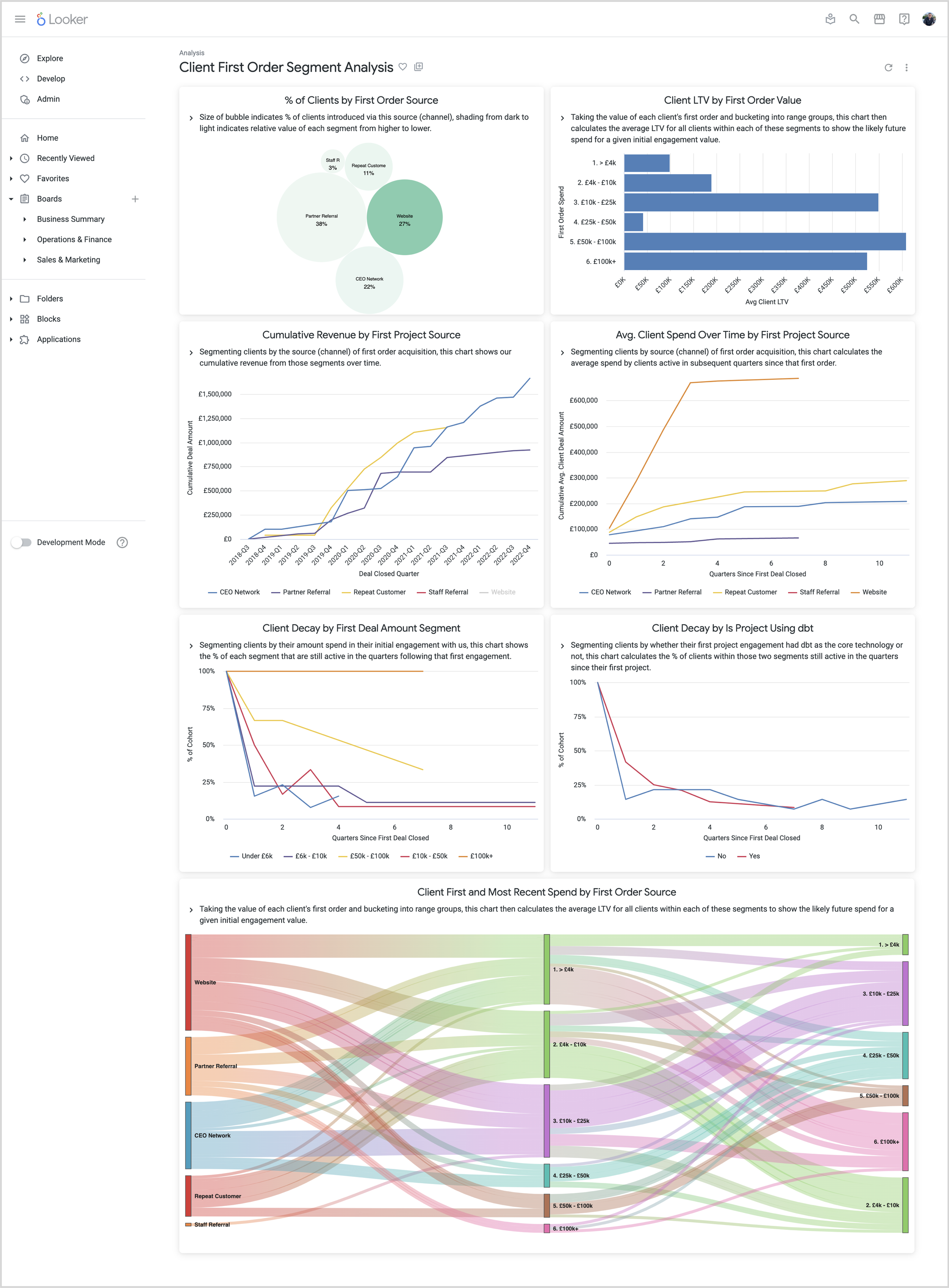
We use first and last order customer segmentation to help us make decisions around which sales channels to invest marketing budget on, which products to base our technology recommendations on and in predicting the future lifetime value of new clients, as shown in the example Looker dashboard below.
Segmenting your customers by first order in a tool such as Looker is a relatively simple process if you’re comfortable with SQL and Looker development, as it will typically involve adding two additional LookML views into your Looker project to calculate:
-
For each customer, the first and last order values for order elements that you’re interested in – product category ordered, sales channel for that order, etc
-
For each transaction, the months, quarters and weeks that the transaction date was from that customer’s first order
My usual method for creating these two LookML views is to first create a Looker query that returns all customer orders, one row per order, with all of the fields you want to segment by and also the customer and transaction keys, so that we can join the final LookML views back into our LookML model at the end.
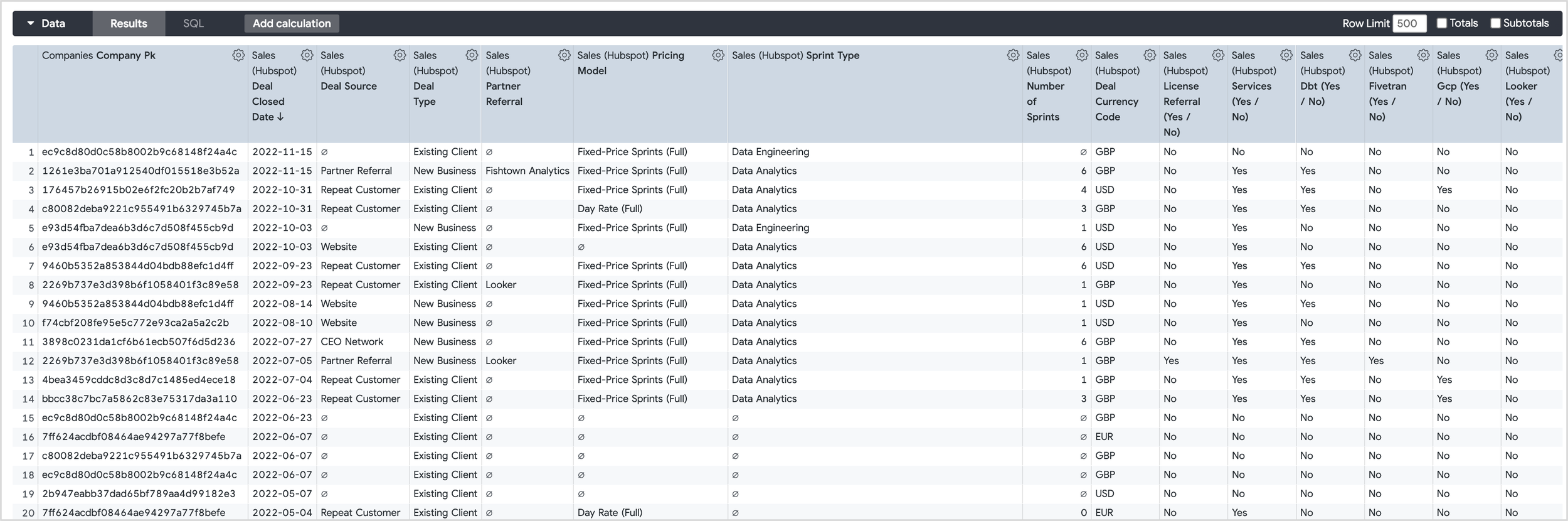
Then I’d click on the SQL button in the explore Data panel to show the SQL that Looker generated, which would typically look like the example below for a Google BigQuery data warehouse data source:
SELECT
companies_dim.company_pk AS companies_dim_company_pk,
(DATE(deals_fact.deal_closed_ts)) AS deals_fact_deal_closed_date,
deals_fact.deal_source AS deals_fact_deal_source,
deals_fact.deal_partner_referral AS deals_fact_partner_referral,
deals_fact.deal_pricing_model AS deals_fact_pricing_model,
...
FROM `analytics.companies_dim` AS companies_dim
LEFT JOIN `analytics.deals_fact` AS
deals_fact ON companies_dim.company_pk = deals_fact.company_pk
WHERE (deals_fact.pipeline_stage_closed_won )
GROUP BY
1,2,3,4,5...
To turn this into a query that calculates the first order value for those columns for each customer, I’d use the FIRST_VALUE () OVER () analytic function to return those first order values and then wrap the query results in a GROUP BY aggregation to return just one row per customer, after first removing transaction date from the results, like this:
WITH deals AS
(SELECT
companies_dim.company_pk AS companies_dim_company_pk,
first_value(deals_fact.deal_source) over
(partition by companies_dim.company_pk order by deals_fact.deal_closed_ts)
AS is_first_deal_license_referral,
first_value(deal_partner_referral) over
(partition by companies_dim.company_pk order by deals_fact.deal_closed_ts)
AS is_first_deal_services,
first_value(deal_pricing_model) over
(partition by companies_dim.company_pk order by deals_fact.deal_closed_ts)
AS is_first_deal_dbt,
...
FROM
`analytics.deals_fact` AS deals_fact
JOIN
`analytics.companies_dim` AS companies_dim ON deals_fact.company_pk = companies_dim.company_pk
WHERE
deals_fact.pipeline_stage_closed_won
)
SELECT
*
FROM
deals
GROUP BY
1,2,3,4...
Taking the same initial order-level Looker query and then reducing it to just the order key and transaction date, I can then use the FIRST_VALUE analytic function along with the BigQuery DATE_DIFF function to calculate months, quarters and years since each customers’ first order date:
with transactions as (SELECT
deals_fact.deal_pk,
first_value(deal_closed_ts) over
(partition by company_pk order by deal_closed_ts) as first_deal_closed_ts,
date_diff(date(deal_closed_ts),first_value(date(deal_closed_ts)) over (partition by company_pk order by deal_closed_ts),MONTH) as months_since_first_deal_closed,
date_diff(date(deal_closed_ts),first_value(date(deal_closed_ts)) over (partition by company_pk order by deal_closed_ts),QUARTER) as quarters_since_first_deal_closed,
date_diff(date(deal_closed_ts),first_value(date(deal_closed_ts)) over (partition by company_pk order by deal_closed_ts),YEAR) as years_since_first_deal_closed
FROM
`analytics.deals_fact` AS deals_fact
WHERE
deals_fact.pipeline_stage_closed_won
)
SELECT
*
FROM
transactions
;;
Note that for this second SQL query, we do not need to aggregate the rows it returns as we want to join it back into our Looker model at the individual transaction level.
Finally I then create two new LookML views based on these queries as the source for their derived table SQL, and then join them back to the existing LookML customer and transaction views within in my LookML model at the individual customer and transaction level, like this:
join: customer_first_deal_cohorts {
view_label: " Sales (Hubspot)"
sql_on: ${deals_fact.deal_pk} =
${customer_first_deal_cohorts.deal_pk};;
type: inner
relationship: one_to_one
}
join: customer_first_order_segments {
view_label: ” Companies”
sql_on: ${companies_dim.company_pk} =
${customer_first_order_segments.companies_dim_company_pk} ;;
type: left_outer
relationship: one_to_one
}
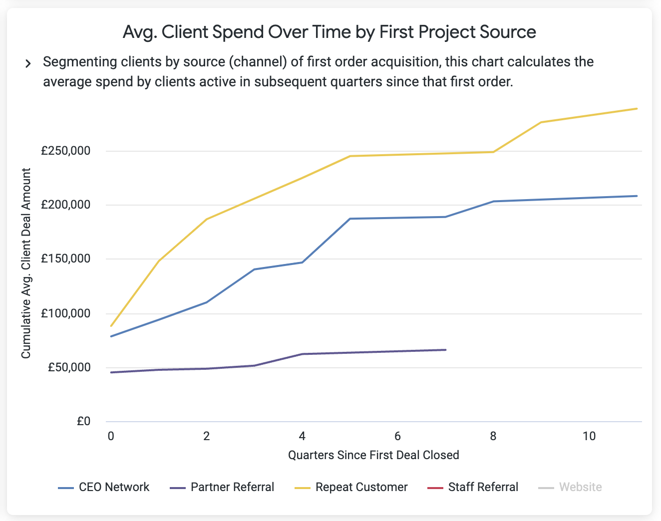
.. and now I can start creating my Looker dashboard visualisations. Most of the charts are a variation on the one below which charts the average spend for each segment of customers indexed by quarters since their first order.
All of these visualizations use a set of common Looker table positional and running total calculations such as the ones in the example screenshot below, with each individual visualisation using particular selections of those calculations.
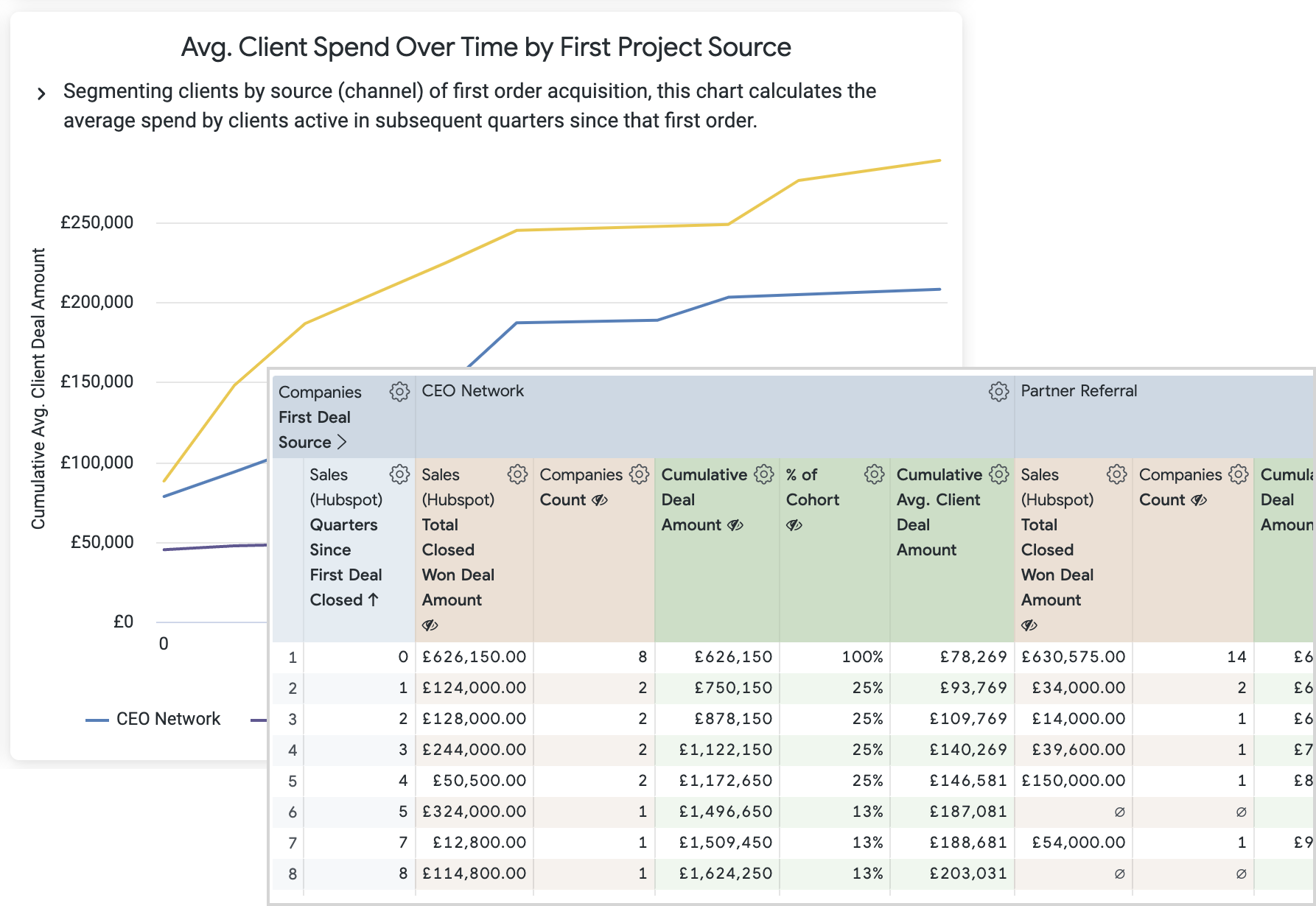
For example, another variation on this visualization are the Client decay visualizations in the main dashboard at the start of the article where the initial 100% population of each segment at the time of their first order is then recalculated each quarter after that first order to show the % still active (i.e. have ordered) after that time, using a table calculation such as:
(${companies_dim.count} / index(${companies_dim.count},1))
And finally, if you’re wondering about the final final visualization on the dashboard showing customer spend on projects at the start and end of their engagement with us, it uses Sankey visualization type that you can install from the Looker Marketplace – useful also for customer journey-type data visualizations.
INTERESTED? FIND OUT MORE
Rittman Analytics is a boutique analytics consultancy specializing in the modern data stack who can help you centralise your data sources, optimize your marketing activity and enable your end-users and data team with best practices and a modern analytics workflow.
If you’re looking for some help and assistance analyzing and understanding your customer behaviour, or to help build-out your analytics capabilities and data team using a modern, flexible and modular data stack, contact us now to organize a 100%-free, no-obligation call — we’d love to hear from you!
CEO of Rittman Analytics, host of the Drill to Detail Podcast, ex-product manager and twice company founder.
Recommended Posts
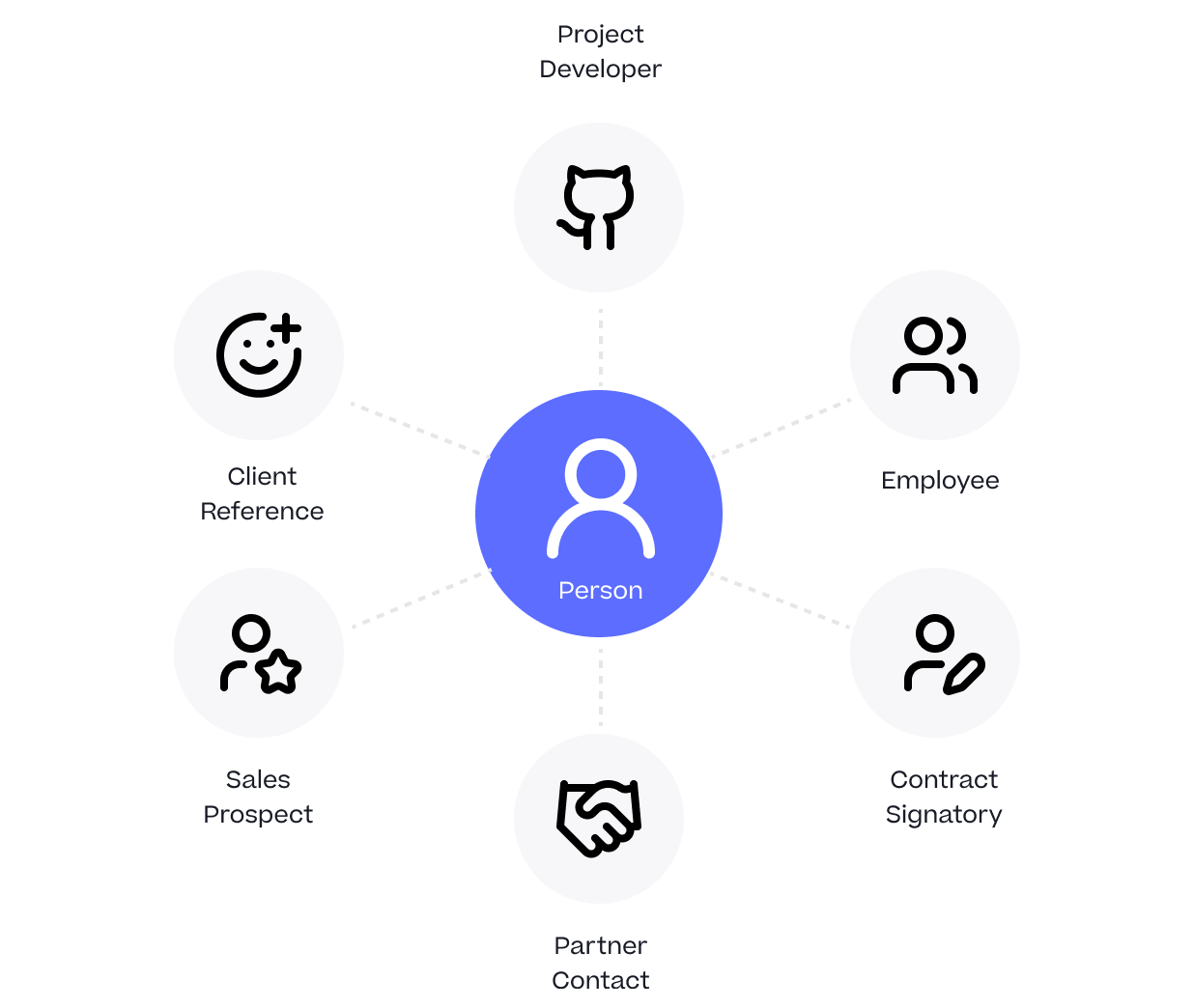
One Person Many Roles: Designing a Unified Person Dimension in Google BigQuery
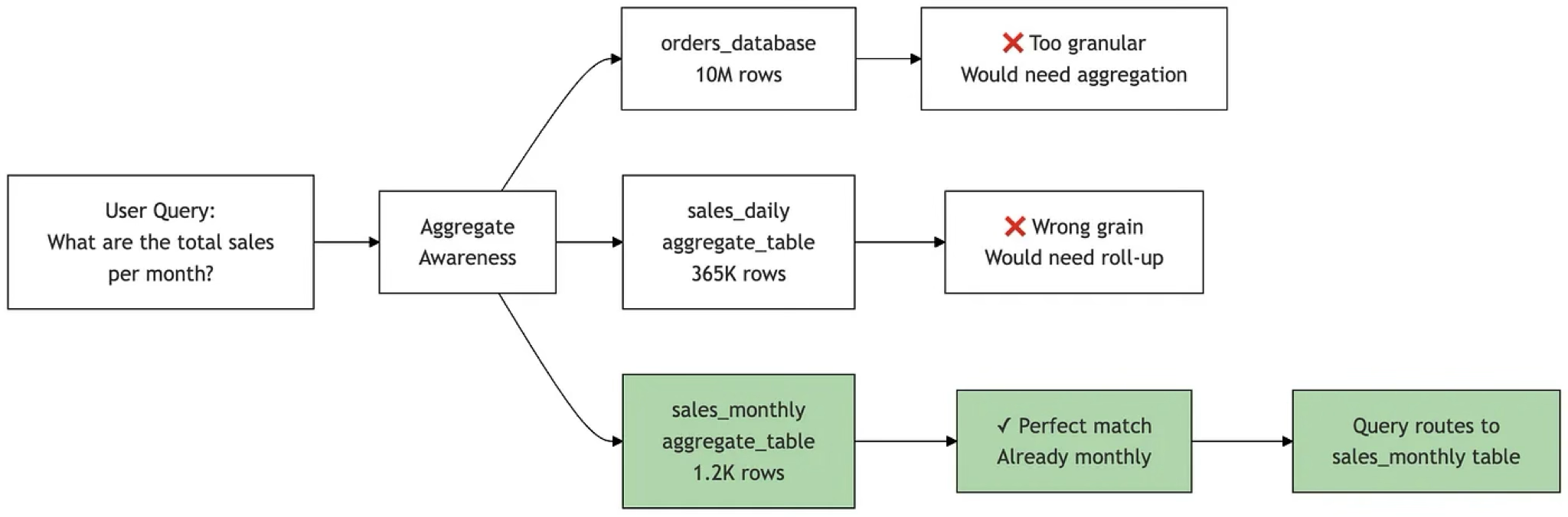
Adventures in Aggregate Awareness (and Level-Specific Measures) with Looker
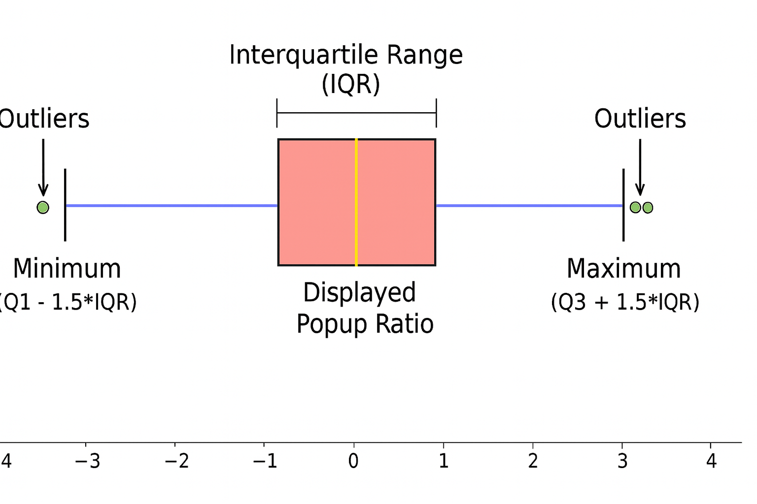
IQR-Based Website Event Anomaly Detection using Looker and Google BigQuery — Rittman Analytics